確率分布について解説します。
この範囲は「データサイエンティストのためのスキルチェックリスト」の「データサイエンス力」項目No.10の解説になります。
多くの専門用語や公式が登場しますが丁寧に理解しやすく説明していきます。
本記事はデータサイエンスを研究されているIffat Maabさんによる英語の解説を翻訳しています。
Iffat Maab
東京大学大学院工学系研究科技術経営戦略学専攻(TMI)博士課程在学中。パキスタン、イスラマバード市出身
マーケターのためのデータサイエンスの時間とは?
こちらの講座では、一般社団法人データサイエンティスト協会様がリリースしている「データサイエンティストのためのスキルチェックリスト」に沿った解説を行っていきます。
「データサイエンティストのためのスキルチェックリスト」とは、データサイエンティストとして活躍するために必要なスキルが体系化されたものです。

このマーケターのためのデータサイエンスの時間に従って学習していくと、データサイエンティストに必要なスキルセットである「データサイエンス力」を一通り学習することが出来ます。
<マーケターのためのデータサイエンスの時間の全一覧はこちら>
5つ以上の代表的な確率分布を説明できる
解答
代表的な確率分布として「離散確率分布」と「連続確率分布」が挙げられ、後述で特徴が記載されています。
解説
はじめに|確率分布とは
確率分布とは、全ての事象の確率を分かりやすく表したものになります。
例えば、サイコロの目の確率分布は以下のようになります。
| サイコロの目 | 確立 |
| 1 | 1/6 |
| 2 | 1/6 |
| 3 | 1/6 |
| 4 | 1/6 |
| 5 | 1/6 |
| 6 | 1/6 |
| 合計 | 1 |
試行の結果として定まる変数によって確立分布は異なります。
具体的には、その変数を連続変数の確率で定義するか,離散変数の確率で定義するかによって、連続確率分布と離散確率分布に分けられます。
突然新しい言葉が出てきましたが、それぞれの定義については以下の通りです。
離散変数: 間の数を数えられない数値型の変数。
例. サイコロの目が離散変数に当てはまります。1と2の目の間に1.4がなく、間の数を数えられません。
連続変数: 間に無限の数を持つ数値型の変数。
例. 身長が当てはまります。連続する180cmと181cmの間には180.1cmや180.1219cmなどがあり無限の値を取ることが出来ます。
そして、どちらの確率分布にも共通する特徴は以下の通りになります。
- 確率のすべての可能な値の合計は1になる。
- 確率の範囲の値は常に0から1の間でなければならず,1に近づくほど確立が高く,離れるほど低い確率を示す。
これらの特徴は当たり前のようなことですが確率分布を理解する上では重要になります。
それでは、代表的な2つの確立分布の特徴を説明します。
①離散確率分布の特徴
離散確率分布は,離散変数の各値の発生確率を記述したものです。
離散変数は上記で説明したように、間の数を数えられない数値型の変数のことを指します。
離散確率分布では,離散確率変数の各可能値は,ゼロではない確率と関連付けることができます。そのため,離散確率分布は,しばしば表形式で示されます。
離散確率分布関数には2つの特徴があります。
- 各確率は0と1の間にある。
- 確率の合計は1に等しい。
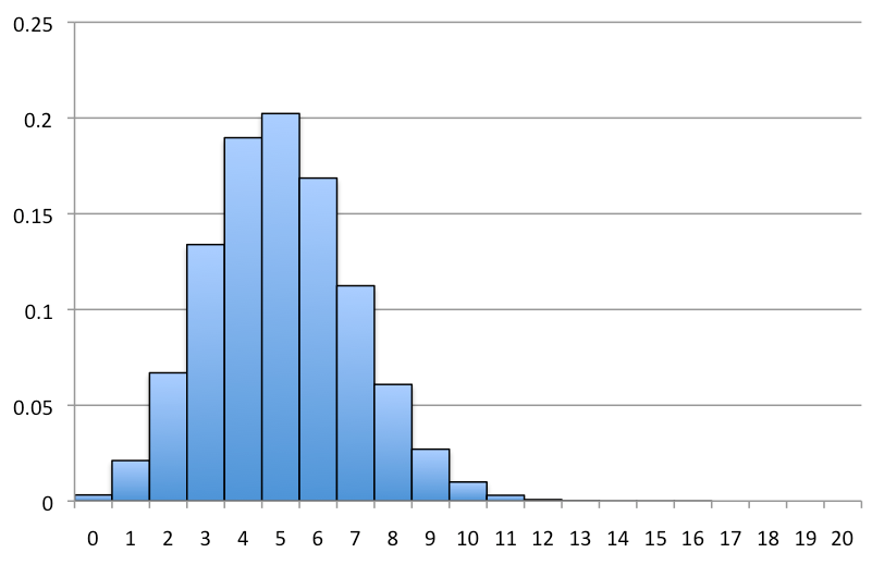
Statics|(Discrete) Probability Distributions
②連続確率分布の特徴
連続確率分布は、連続変数の可能な値の確率を記述します。
連続変数は上記で説明したように、身長や体重のような数値間に無限の数を持つ数値型の変数のことを指します。
連続確率分布は、以下のような確率密度関数の曲線の下の面積として定義されます。
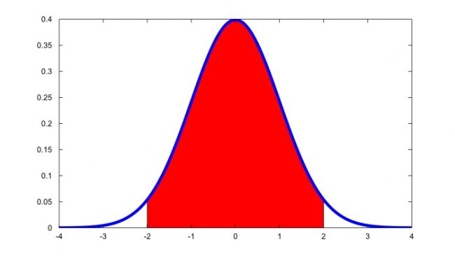
確率密度関数とは、連続確立変数がある値をとる確率密度を関数にしたものです。
連続確率変数では、それがある区間に存在する確率を考えなければなりません。この結果の重要性は、確率を求めるためには、与えられた区間の連続確立変数の下の面積を求める必要があることを教えてくれることです。
- 連続確立変数の下の面積の合計は1になります。(上の図では赤い部分の面積)
この結果は,確率変数が与えられた区間に存在する確率を近似するためには,区間の両端間の連続確立変数の下の面積の割合を推測すればよいことを意味しています。
まとめ
以上が「データサイエンス力」のNo.10の解説になります。

English
Explain 5 or more characteristics of typical probability distributions
Probability distributions tell the likelihood (chance) of an event. Usually statisticians use the following notation to describe probability:
p(x) = the likelihood that a random variable takes a specific value of x.
Probability distributions are either continuous probability distributions or discrete probability distributions, depending on whether they define probabilities for continuous or discrete variables [1].
Following are some characteristics of probability distributions [2]:
- The sum of all possible values of a probability is equal to 1.
- The probability range value must be always between 0 and 1. The lowest probability while 1 shows the highest probability value.
- In probability theory and statistics, a probability distribution is the mathematical function that gives the probabilities of occurrence of different possible outcomes for an experiment. It is a mathematical description of a random phenomenon in terms of its sample space and the probabilities of events.
- Discrete probability functions are also known as probability mass functions and can assume a discrete number of values. For example, coin tosses and counts of events are discrete functions.
- Probability distributions describe the dispersion of the values of a random variable. Consequently, the kind of variable determines the type of probability distribution. For a single random variable, statisticians divide distributions into the following two types:
- Discrete probability distributions for discrete variables.
- Probability density functions for continuous variables.
Discrete probability distribution
A discrete distribution describes the probability of occurrence of each value of a discrete random variable. A discrete random variable is a random variable that has countable values, such as a list of non-negative integers for example number of customer complaints [1].
With a discrete probability distribution, each possible value of the discrete random variable can be associated with a non-zero probability. Thus, a discrete probability distribution is often presented in tabular form
A discrete probability distribution function has two characteristics:
- Each probability is between zero and one, inclusive (inclusive means to include zero and one).
- The sum of the probabilities is equal to one.
Continuous probability distribution
A continuous probability distribution describes the probabilities of the possible values of a continuous random variable. A continuous random variable is a random variable with a set of possible values (known as the range) that is infinite and uncountable.
Probabilities of continuous random variables (X) are defined as the area under the curve of its PDF. The characteristic and significance of PDF are [3]:
- For a continuous random variable, one must consider the probability that it lies in an interval. The importance of this result is that it tells us that, to find the probability, we need to find the area under the pdf on the given interval.
- The total area under the pdf equals 1. This result means that in order to approximate the probability that the random variable lies in a given interval, we just have to guess the fraction of the area under the pdf between the ends of the interval. This result provides another perspective on why pdfs cannot be negative, since if they were, a negative probability could be obtained, which is impossible (i.e., area cannot be negative).
著者情報