標準正規分布について解説します。
この範囲は「データサイエンティストのためのスキルチェックリスト」の「データサイエンス力」項目No.6の解説になります。
多くの専門用語や公式が登場しますが丁寧に理解しやすく説明していきます。
本記事はデータサイエンスを研究されているIffat Maabさんによる英語の解説を翻訳しています。
Iffat Maab
東京大学大学院工学系研究科技術経営戦略学専攻(TMI)博士課程在学中。パキスタン、イスラマバード市出身
マーケターのためのデータサイエンスの時間とは?
こちらの講座では、一般社団法人データサイエンティスト協会様がリリースしている「データサイエンティストのためのスキルチェックリスト」に沿った解説を行っていきます。
「データサイエンティストのためのスキルチェックリスト」とは、データサイエンティストとして活躍するために必要なスキルが体系化されたものです。

このマーケターのためのデータサイエンスの時間に従って学習していくと、データサイエンティストに必要なスキルセットである「データサイエンス力」を一通り学習することが出来ます。
標準正規分布の分散と平均の値を知っている
解答
標準正規分布の分散は1、平均は0である。
解説
標準正規分布
標準正規分布とは確率分布の1種で、平均(μ)がゼロ,分散(σ²)が単位である分布のことです。
ここで、母平均はμ(ミュー)、母分散はσ²(シグマ)で表されます。
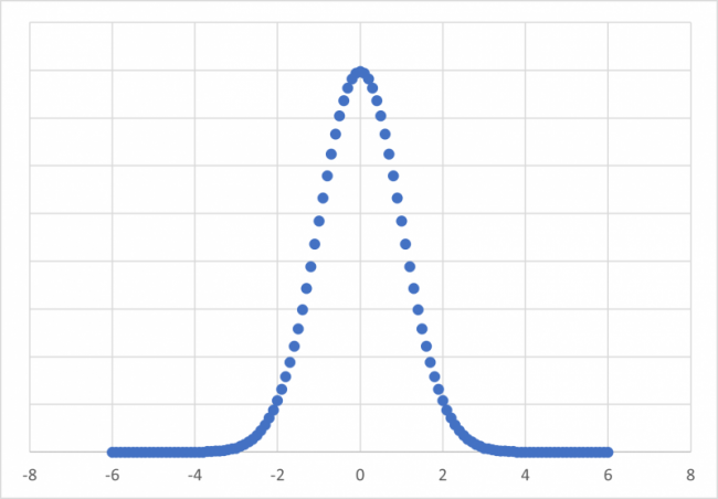
標準正規分布はベル型をしており、平均0を中心にして対称となります。
平均μと分散σ²については、こちらの第6回で説明しています。

標準正規分布で平均と分散がどのように用いられているか
先ほども述べたように、「標準正規分布では、平均が0、分散が1」となっています。
上の分布のようにデータの密度としては、平均付近に非常に集中しており、分布の中心から左右に移動すると非常に小さくなることが分かると思います。
つまり、分布の中心から離れれば離れるほど、その値が観測される可能性は低くなっています
このように可視化することで特に大量のデータを扱う問題では、正規分布を用いて理解しやすくなっています。
その為、平均μと分散σ²を指定し、μとσ²をパラメータとし標準正規分布を固定しているのです。
µを増加させると、正規分布はベル型の外観を変えずに右に移動し、一方、分散σ²を増加させると、密度関数の位置を変えずに平坦になります。
先ほどの表では一部しか表されていませんが、正規分布はマイナスの無限大からプラスの無限大までがあります。
標準正規分布を用いることで分かりやすくなるデータの例
平均と分散で標準正規分布を固定していることが分かったので、次に例を挙げて理解を深めましょう。
例えば、人の身長は、遺伝、栄養(単に良いか悪いかではなく、その人が成長している間に毎日実際に食べられたもの)、環境など、多くの小さな影響によって決定されます。
そのため、(さらに性・人種の組み合わせを考慮しても)身長というデータはほぼ正常で分布されます。
他にも、特定の地域の年間降水量では、その年の毎日の降水量の合計であり、毎日の降水量はおそらく正常から非常にかけ離れていますが、それらの日をすべて合計すると正常な確立分布が得られます。
目的
このように、経済学者や統計学者はデータを数値だけでなく可視化して理解しようとします。
以前の講座で解説したように、平均値はデータの中心傾向を示す尺度です。そして、分散に関しても、統計学者がデータの分散を見るために使用します。
このような平均と分散という2つのパラメータを用いて正規分布に用いることで、データの可視化の幅が広がります。
まとめ
以上が「データサイエンス力」のNo.6の解説になります。

次回はNo.7からの解説になります。1~271項目まで順に追って解説していくので、マーケターの皆さんは本シリーズを読んで、データサイエンスの世界に踏み出していきましょう。
English
A standard normal distribution is a distribution with zero mean and unit variance, given by the probability density function (pdf) and distribution function
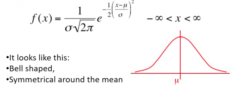
where the population mean will be denoted by µ (pronounced as mew), the population variance by σ2 (pronounced as sigma square). Mean µ and variance σ2 are explained in point # 7. In particular, the standard normal distribution has 0 mean with variance equal to 1. The density is very concentrated around the mean and becomes very small by moving from the center to the left or to the right of the distribution (called “tails” of the distribution). This means that the further a value is from the center of the distribution, the less probable it is to observe that value. A broad range of problems particularly those involving large amounts of datasets can be solved using normal distribution.
We specify mean µ and variance σ2 to fix a particular normal distribution where µ and σ2 are called the parameters of a normal distribution. Increasing µ shifts the normal distribution towards its right without changing its bell shaped appearance whereas increasing the variance σ2 flattens the density function without changing its position. The normal distribution is bell shaped and is symmetric around the mean. Normal distribution runs from minus infinity to the positive infinity.
For example
A person’s height is determined by many small effects including genetics (there will be several genes that contribute to height), nutrition (not just good/ bad, but what was actually eaten each day that the person was growing), environmental pollution (again each day contributed a small effect), and other things. Hence, heights (within sex/race combinations) are approximately normal [8d].
Annual rainfall for a specific area is the summation of the daily rainfall for the year and while the daily rainfall is probably very far from normal (zero inflated) when you add all those days together you get something much more normal.
Purpose
Economists and statisticians often want to describe data in terms of numbers rather than figures. The mean (or average) is a measure of the central tendency of the data. A second parameter which is a variance is used by statisticians to see the dispersion of the data.
Similarly, it is entirely characterized by two parameters i.e., mean and variance that are easy to estimate. Normality assumptions frequently result in analytic (as opposed to numeric) solutions to many estimation problems e.g., from a random sample of 400 citizens in Ottawa, there were 136 who indicated that the city’s transportation system is adequate. Using normal distribution, a confidence interval for the population proportion who feel the transportation system is adequate can be calculated.
References
[8a]https://slideplayer.com/slide/7828801/
[8b]https://saylordotorg.github.io/text_microeconomics-theory-through-applications/s21-22-mean-and-variance.html
[8c]https://courses.lumenlearning.com/introstats1/chapter/the-standard-normal-distribution/
[8d]https://stats.stackexchange.com/questions/49212/importance-of-normal-distribution
著者情報